Image Classification with Convolution Neural Network
Learned how to implement image classification with the three image types using the three popular image datasets: CIFAR, ORL, and MNIST.
Table of contents
Dataset
Dataset Size
There are three datasets for this stage of the project: MNIST, ORL, and CIFAR, which are all image datasets.
- MNIST (gray image)
Training set size: 60,000, testing set size: 10,000, number of classes: 10. Each instance is a 28x28 gray image, and will have one single class label denoted by an integer from {0, 1, …, 9}.
- ORL (gray image)
Training set size: 360, testing set size: 40, number of classes: 40. Each instance is a 112x92 gray image, and will have one single class label denoted by an integer from {1, 2, …, 39, 40}.
- CIFAR (color image)
Training set size: 50,000, testing set size: 10,000, number of classes: 10. Each instance is a 32x32 color image, and will have one single label denoted by an integer from {0, 1, 2, …, 9}.
Dataset Organization
These dataset are organized as with a dictionary data structure in Python as follows:
{
    ‘train’: [
        {‘image’: a matrix/tensor representing a image, ‘label’: an integer representing the label}
        {‘image’: a matrix/tensor representing a image, ‘label’: an integer representing the label}
        …
        {‘image’: a matrix/tensor representing a image, ‘label’: an integer representing the label}
    ],
    ‘test’: [
        {‘image’: a matrix/tensor representing a image, ‘label’: an integer representing the label}
        {‘image’: a matrix/tensor representing a image, ‘label’: an integer representing the label}
        …
        {‘image’: a matrix/tensor representing a image, ‘label’: an integer representing the label}
    ]
}
Abstract
Trained a CNN for these three datasets, respectively, and evaluate its performance on the testing set.
Model
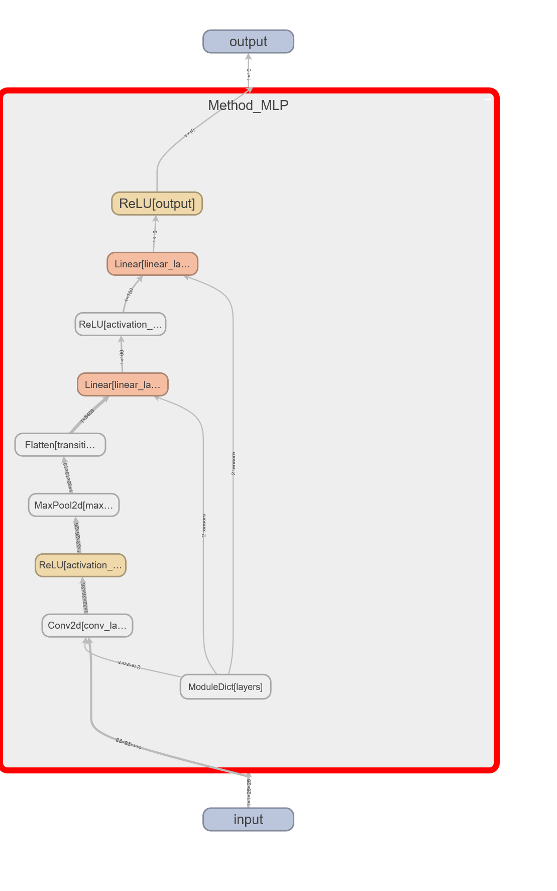
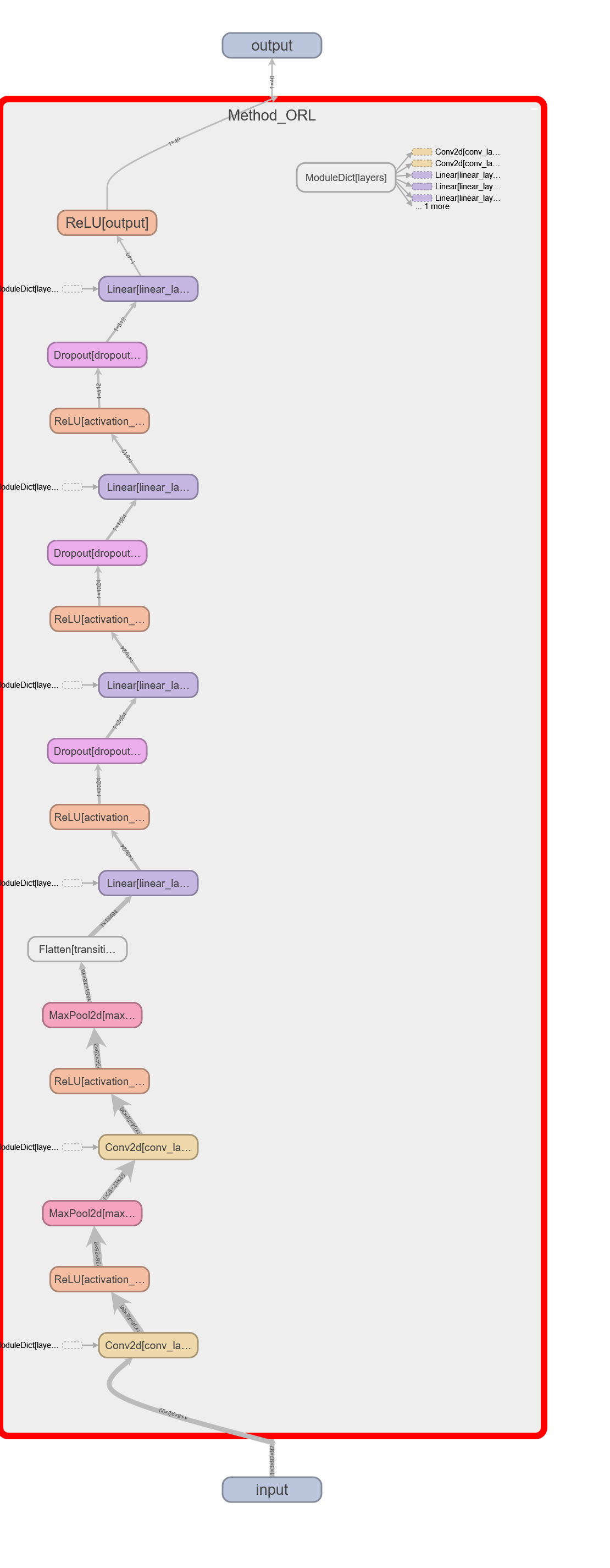
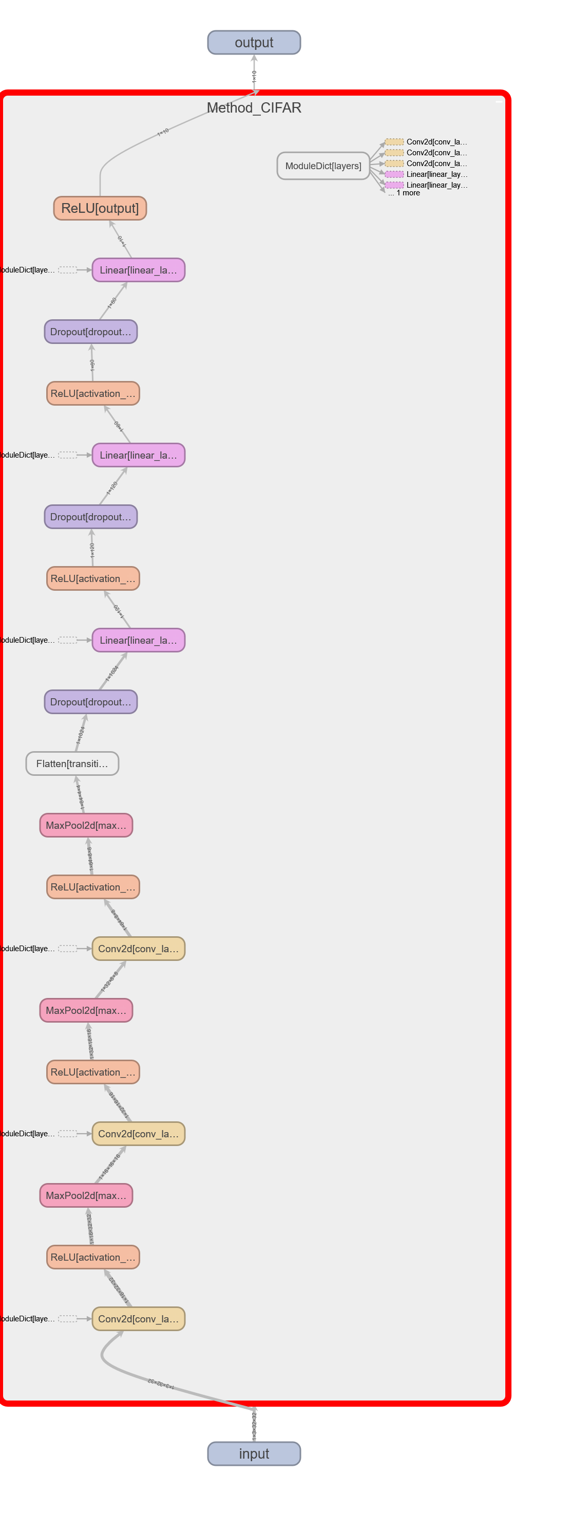
The model in stage 3 uses a simple Convolution Neural Network, ReLu activation layer, MaxPool layer, and fully connected layers at the end. Just like we had in Stage 2, we didn’t use the SoftMax layer at the end due to having the CrossEntropy Loss function. By using the PyTorch library, we found out that the color channel dimension is the last dimension in the input tensor of the OLR and the CIFAR. Since the PyTorch convolution layer only takes in image tensors with format B x C x W x H, we had to swap the dimension position before training. We also use mini-batch in all our training since there is a lot of data.
MNIST Model

ORL Model

CIFAR Model

Experiment
The dataset used in the project is shown to be a handwritten number image dataset. The data was given already split up into train and test. There are three datasets for this stage of the project: MNIST, ORL, and CIFAR, which are all image datasets. MNIST (gray image) is a training set of size 60,000, a testing set of size 10,000, number of classes of 10. Each instance is a 28x28 gray image and will have one single class label denoted by an integer from {0, 1, …, 9}. Those integers each indicate the grayness of the pixel. ORL(gray image) is a dataset of face images consisting of 400 images of 40 individuals, with 10 images per individual. Each image is a grayscale 92x112 pixel image, and the task is to classify each image into one of 40 classes, corresponding to the individuals in the dataset. Since this ORL dataset label index starts at 1 unlike the other 2 datasets, it threw an index out-of-bounds error when we tried to run the code. We had to modify the index so that the code runs without an error. CIFAR (color image) has a training set the size of 50,000, a testing set the size of 10,000, number of classes of 10. Each instance is a 32x32 color image and will have one single label denoted by an integer from {0, 1, 2, …, 9}. The dataset consists of RGB matrices with each matrix having a pixel indicating the opacity of each Red, Green, and Blue color.
Detailed Experiment Setups
Here are the print out details of each layers input, output, and more for each of our models.
MNIST
===================================================================================
Layer (type:depth-idx)                   Output Shape              Param #
===================================================================================
Method_MINST                               [1, 10]                     --
├─ModuleDict: 1-1                        --                        --
│    └─Conv2d: 2-1                       [1, 32, 26, 26]           320
│    └─ReLU: 2-2                         [1, 32, 26, 26]           --
│    └─MaxPool2d: 2-3                    [1, 32, 13, 13]           --
│    └─Flatten: 2-4                      [1, 5408]                 --
│    └─Linear: 2-5                       [1, 100]                  540,900
│    └─ReLU: 2-6                         [1, 100]                  --
│    └─Linear: 2-7                       [1, 10]                   1,010
│    └─ReLU: 2-8                         [1, 10]                   --
ORL
==========================================================================================
Layer (type:depth-idx)                   Output Shape              Param #
==========================================================================================
Method_ORL                               [1, 40]                   --
├─ModuleDict: 1-1                        --                        --
│    └─Conv2d: 2-1                       [1, 36, 86, 86]           5,328
│    └─ReLU: 2-2                         [1, 36, 86, 86]           --
│    └─MaxPool2d: 2-3                    [1, 36, 43, 43]           --
│    └─Conv2d: 2-4                       [1, 54, 39, 39]           48,654
│    └─ReLU: 2-5                         [1, 54, 39, 39]           --
│    └─MaxPool2d: 2-6                    [1, 54, 19, 19]           --
│    └─Flatten: 2-7                      [1, 19494]                --
│    └─Linear: 2-8                       [1, 2024]                 39,457,880
│    └─ReLU: 2-9                         [1, 2024]                 --
│    └─Dropout: 2-10                     [1, 2024]                 --
│    └─Linear: 2-11                      [1, 1024]                 2,073,600
│    └─ReLU: 2-12                        [1, 1024]                 --
│    └─Dropout: 2-13                     [1, 1024]                 --
│    └─Linear: 2-14                      [1, 512]                  524,800
│    └─ReLU: 2-15                        [1, 512]                  --
│    └─Dropout: 2-16                     [1, 512]                  --
│    └─Linear: 2-17                      [1, 40]                   20,520
│    └─ReLU: 2-18                        [1, 40]                   --
==========================================================================================
Total params: 42,130,782
Trainable params: 42,130,782
Non-trainable params: 0
Total mult-adds (M): 155.49
==========================================================================================
Input size (MB): 0.10
Forward/backward pass size (MB): 2.82
Params size (MB): 168.52
Estimated Total Size (MB): 171.44
CIFAR
==========================================================================================
Layer (type:depth-idx)                   Output Shape              Param #
==========================================================================================
Method_CIFAR                             [1, 10]                   --
├─ModuleDict: 1-1                        --                        --
│    └─Conv2d: 2-1                       [1, 16, 32, 32]           448
│    └─ReLU: 2-2                         [1, 16, 32, 32]           --
│    └─MaxPool2d: 2-3                    [1, 16, 16, 16]           --
│    └─Conv2d: 2-4                       [1, 32, 16, 16]           4,640
│    └─ReLU: 2-5                         [1, 32, 16, 16]           --
│    └─MaxPool2d: 2-6                    [1, 32, 8, 8]             --
│    └─Conv2d: 2-7                       [1, 64, 8, 8]             18,496
│    └─ReLU: 2-8                         [1, 64, 8, 8]             --
│    └─MaxPool2d: 2-9                    [1, 64, 4, 4]             --
│    └─Flatten: 2-10                     [1, 1024]                 --
│    └─Dropout: 2-11                     [1, 1024]                 --
│    └─Linear: 2-12                      [1, 120]                  123,000
│    └─ReLU: 2-13                        [1, 120]                  --
│    └─Dropout: 2-14                     [1, 120]                  --
│    └─Linear: 2-15                      [1, 60]                   7,260
│    └─ReLU: 2-16                        [1, 60]                   --
│    └─Dropout: 2-17                     [1, 60]                   --
│    └─Linear: 2-18                      [1, 10]                   610
│    └─ReLU: 2-19                        [1, 10]                   --
==========================================================================================
Total params: 154,454
Trainable params: 154,454
Non-trainable params: 0
Total mult-adds (M): 2.96
==========================================================================================
Input size (MB): 0.01
Forward/backward pass size (MB): 0.23
Params size (MB): 0.62
Estimated Total Size (MB): 0.86
==========================================================================================
We modified the Method_ORL/Method_MINST/Method_CIFAR class using OrderedDict() to organize our layers so that we can easily add more hidden layers and gather training data on different architectures more effectively.
For our hyperparameters, we have our learning rate at 1e-3 and our momentum at 0.9. We train our model with 1000 epochs and set the manual random seed to 42. We currently don’t use any special initialization method for the weight in our layer and rely on the layer default initialization. In the beginning, we developed our network following AlexNet architecture. However, the time it takes to train one single dataset on AlexNet deems it unfathomable for us to accomplish in less than a week. We decided to cut down and use mainly only 2-3 convolution layers in our features learning group.
We also found out through experiments and research that using SGD is better than ADAM when used for Image Classification tasks (source: https://opt-ml.org/papers/2021/paper53.pdf). The ORL dataset gave us the biggest trouble because of its non-square image size and the label data does not start at 0. We train our network on GPU using the CUDA library. We found out after keep receiving runtime errors and found out that the library wants the data label to start at 0 instead of 1, thus we have to modify the dataset more than the other two.
Evaluation Metrics
We use scikit-learn library’s classification_report() function to report F1, Accuracy, precision and recall when using our test dataset.
MNIST Training Result
 MNIST Model Performance
method running...
--start training...
Epoch: 0 Accuracy: 0.385 Loss: 1.76118803024292
Epoch: 100 Accuracy: 0.89 Loss: 0.25425952672958374
Epoch: 200 Accuracy: 0.9 Loss: 0.23050585389137268
Epoch: 300 Accuracy: 0.904 Loss: 0.22125254571437836
Epoch: 400 Accuracy: 0.906 Loss: 0.21649625897407532
Epoch: 500 Accuracy: 0.879 Loss: 0.27869507670402527
Epoch: 600 Accuracy: 0.905 Loss: 0.21881769597530365
Epoch: 700 Accuracy: 0.919 Loss: 0.1888771951198578
Epoch: 800 Accuracy: 0.899 Loss: 0.2325960248708725
Epoch: 900 Accuracy: 0.88 Loss: 0.27634069323539734
--start testing...
run performance metrics:
...
              precision    recall  f1-score   support

           0       0.50      0.99      0.67       980
           1       0.99      0.99      0.99      1135
           2       0.98      0.99      0.98      1032
           3       0.98      0.99      0.98      1010
           4       0.00      0.00      0.00       982
           5       0.98      0.98      0.98       892
           6       0.98      0.98      0.98       958
           7       0.97      0.98      0.97      1028
           8       0.97      0.98      0.98       974
           9       0.97      0.97      0.97      1009

    accuracy                           0.89     10000
   macro avg       0.83      0.88      0.85     10000
weighted avg       0.84      0.89      0.85     10000

saving results...
saving models...
Accuracy is: 88.63%
ORL Training Result
 ORL Model Performance
--start training...
Epoch: 0 Accuracy: 0.016666666666666666 Loss: 3.7312941551208496
Epoch: 100 Accuracy: 1.0 Loss: 0.011220413260161877
Epoch: 200 Accuracy: 1.0 Loss: 0.002023124136030674
Epoch: 300 Accuracy: 1.0 Loss: 0.00012056121340719983
...
--start testing...
run performace metrics:
              precision    recall  f1-score   support

           0       1.00      1.00      1.00         1
           1       1.00      1.00      1.00         1
           2       1.00      1.00      1.00         1
           3       1.00      1.00      1.00         1
           4       0.00      0.00      0.00         1
           5       1.00      1.00      1.00         1
           6       1.00      1.00      1.00         1
           7       1.00      1.00      1.00         1
           8       1.00      1.00      1.00         1
           9       0.00      0.00      0.00         1
          10       1.00      1.00      1.00         1
          11       1.00      1.00      1.00         1
          12       1.00      1.00      1.00         1
          13       1.00      1.00      1.00         1
          14       1.00      1.00      1.00         1
          15       1.00      1.00      1.00         1
          16       1.00      1.00      1.00         1
          17       1.00      1.00      1.00         1
          18       1.00      1.00      1.00         1
          19       1.00      1.00      1.00         1
          20       1.00      1.00      1.00         1
          21       1.00      1.00      1.00         1
          22       1.00      1.00      1.00         1
          23       1.00      1.00      1.00         1
          24       1.00      1.00      1.00         1
          25       1.00      1.00      1.00         1
          26       1.00      1.00      1.00         1
          27       1.00      1.00      1.00         1
          28       1.00      1.00      1.00         1
          29       1.00      1.00      1.00         1
          30       0.50      1.00      0.67         1
          31       0.50      1.00      0.67         1
          32       1.00      1.00      1.00         1
          33       1.00      1.00      1.00         1
          34       1.00      1.00      1.00         1
          35       0.00      0.00      0.00         1
          36       1.00      1.00      1.00         1
          37       1.00      1.00      1.00         1
          38       1.00      1.00      1.00         1
          39       0.00      0.00      0.00         1

    accuracy                           0.90        40
   macro avg       0.88      0.90      0.88        40
weighted avg       0.88      0.90      0.88        40

saving results...
saving models...
Accuracy is: 90.0%
CIFAR Training Result
 CIFAR Model Performance
--start training...
Epoch: 0 Accuracy: 0.12 Loss: 2.2826151847839355
Epoch: 100 Accuracy: 0.684 Loss: 0.9034884572029114
Epoch: 200 Accuracy: 0.754 Loss: 0.705613911151886
Epoch: 300 Accuracy: 0.791 Loss: 0.5829808115959167
Epoch: 400 Accuracy: 0.843 Loss: 0.480678915977478
Epoch: 500 Accuracy: 0.868 Loss: 0.3825521171092987
Epoch: 600 Accuracy: 0.901 Loss: 0.3389916718006134
Epoch: 700 Accuracy: 0.876 Loss: 0.34137627482414246
Epoch: 800 Accuracy: 0.908 Loss: 0.25142887234687805
Epoch: 900 Accuracy: 0.899 Loss: 0.2848355770111084
--start testing...
run performace metrics:
              precision    recall  f1-score   support

           0       0.71      0.73      0.72      1000
           1       0.81      0.83      0.82      1000
           2       0.61      0.57      0.59      1000
           3       0.50      0.53      0.51      1000
           4       0.69      0.61      0.65      1000
           5       0.58      0.59      0.59      1000
           6       0.78      0.78      0.78      1000
           7       0.75      0.73      0.74      1000
           8       0.82      0.80      0.81      1000
           9       0.74      0.82      0.78      1000

    accuracy                           0.70     10000
   macro avg       0.70      0.70      0.70     10000
weighted avg       0.70      0.70      0.70     10000

saving results...
saving models...
Accuracy is: 69.87%
Ablation Studies
Based on our experience, the ADAM optimizer performs worse than SGD in image classification. Also, our initial thought of using AlexNet architecture seems too difficult because of our time constraints. We also tried to use full batch training at the beginning for all datasets. However, we quickly realized that we ran out of memory from our GPU. Thus we decided to implement our training loop into mini-batches of different sizes depending on the size of the input dataset and the number of dimensions they have.
We also did multiple trains with the CIFAR dataset, using other epoch numbers and utilizing Tensorboard to make sure there are not any symptoms of vanishing gradients during training. We trained using 400, 600, and then 1000 epochs, but we could not get higher than 71% accuracy in our testing result. We suspect there may be a lack of depth in our architecture and think that with a deeper model, we can achieve higher accuracy.
Source Code
GitHub repository page: https://github.com/CyberExplosion/Deep-Learning-Projects/tree/P3